January 1, 2022
Intro
I wanted to analyze and visualize the correlation between electoral college votes for either candidate in the 2016 election against the average total gun violence for each state.
library(dslabs)
# data_frame('murders')
# data_frame('results_us_election_2016')
head(murders)
## state abb region population total
## 1 Alabama AL South 4779736 135
## 2 Alaska AK West 710231 19
## 3 Arizona AZ West 6392017 232
## 4 Arkansas AR South 2915918 93
## 5 California CA West 37253956 1257
## 6 Colorado CO West 5029196 65head(results_us_election_2016)## state electoral_votes clinton trump others
## 1 California 55 61.7 31.6 6.7
## 2 Texas 38 43.2 52.2 4.5
## 3 Florida 29 47.8 49.0 3.2
## 4 New York 29 59.0 36.5 4.5
## 5 Illinois 20 55.8 38.8 5.4
## 6 Pennsylvania 20 47.9 48.6 3.6Joining the Data Sets
library(dplyr)
project <- left_join(murders, results_us_election_2016, by = "state") %>%
    select(-others) %>% rename(ev = electoral_votes)
head(project)
## state abb region population total ev clinton trump
## 1 Alabama AL South 4779736 135 9 34.4 62.1
## 2 Alaska AK West 710231 19 3 36.6 51.3
## 3 Arizona AZ West 6392017 232 11 45.1 48.7
## 4 Arkansas AR South 2915918 93 6 33.7 60.6
## 5 California CA West 37253956 1257 55 61.7 31.6
## 6 Colorado CO West 5029196 65 9 48.2 43.3Summarizing and DPLYR
library(dplyr)
library(dslabs)
library(tidyr)
gbregion <- project %>% group_by(region) %>% summarize_if(is.numeric,
    c(mean = mean, sd = sd))
head(gbregion)
## # A tibble: 4 x 11
## region population_mean total_mean ev_mean clinton_mean trump_mean
## <fct> <dbl> <dbl> <dbl> <dbl> <dbl>
## 1 North… 6146360 163. 10.7 53.7 40.1
## 2 South 6804378. 247. 11.5 44.0 51.6
## 3 North… 5577250. 152. 9.83 40.5 53
## 4 West 5534273. 147 9.85 43.6 45.9
## # … with 5 more variables: population_sd <dbl>, total_sd <dbl>, ev_sd <dbl>,
## # clinton_sd <dbl>, trump_sd <dbl>project %>% group_by(region) %>% summarize_if(is.numeric, c(mean = mean,
sd = sd)) %>% pivot_longer(-region) %>% separate(name, into = c("var",
"stat"))## # A tibble: 40 x 4
## region var stat value
## <fct> <chr> <chr> <dbl>
## 1 Northeast population mean 6146360
## 2 Northeast total mean 163.
## 3 Northeast ev mean 10.7
## 4 Northeast clinton mean 53.7
## 5 Northeast trump mean 40.1
## 6 Northeast population sd 6469174.
## 7 Northeast total sd 200.
## 8 Northeast ev sd 8.94
## 9 Northeast clinton sd 4.94
## 10 Northeast trump sd 6.16
## # … with 30 more rowsfilter(project, region == "south") %>% summarise(mean = mean(project$total))## mean
## 1 184.3725topten <- project %>% arrange(desc(population), .by_group = TRUE) %>%
slice(1:10)
head(topten)## state abb region population total ev clinton trump
## 1 California CA West 37253956 1257 55 61.7 31.6
## 2 Texas TX South 25145561 805 38 43.2 52.2
## 3 Florida FL South 19687653 669 29 47.8 49.0
## 4 New York NY Northeast 19378102 517 29 59.0 36.5
## 5 Illinois IL North Central 12830632 364 20 55.8 38.8
## 6 Pennsylvania PA Northeast 12702379 457 20 47.9 48.6murders <- project %>% mutate(murders, rate = total/population *
1e+05)
head(murders)## state abb region population total ev clinton trump rate
## 1 Alabama AL South 4779736 135 9 34.4 62.1 2.824424
## 2 Alaska AK West 710231 19 3 36.6 51.3 2.675186
## 3 Arizona AZ West 6392017 232 11 45.1 48.7 3.629527
## 4 Arkansas AR South 2915918 93 6 33.7 60.6 3.189390
## 5 California CA West 37253956 1257 55 61.7 31.6 3.374138
## 6 Colorado CO West 5029196 65 9 48.2 43.3 1.292453murders %>% select(state, region, rate) %>% filter(rate <= 0.71)## state region rate
## 1 Hawaii West 0.5145920
## 2 Iowa North Central 0.6893484
## 3 New Hampshire Northeast 0.3798036
## 4 North Dakota North Central 0.5947151
## 5 Vermont Northeast 0.3196211## using summarize
us_murder_rate <- project %>% summarize(rate = sum(total)/sum(population) *
1e+05)
us_murder_rate## rate
## 1 3.034555summarize(project, mean(population))## mean(population)
## 1 6075769project %>% filter(region == "south") %>% summarize(average = mean(project$trump,
na.rm = T), standard_deviation = sd(project$trump, na.rm = TRUE))## average standard_deviation
## 1 48.45098 11.95812project %>% group_by(region) %>% summarize(median = median(clinton),
minimum = min(clinton), maximum = max(clinton))## # A tibble: 4 x 4
## region median minimum maximum
## <fct> <dbl> <dbl> <dbl>
## 1 Northeast 54.6 46.8 60
## 2 South 40.7 26.5 90.9
## 3 North Central 39.9 27.2 55.8
## 4 West 47.9 21.9 62.2project %>% group_by(region) %>% summarize(range = quantile(ev,
c(0, 0.5, 1)))## # A tibble: 12 x 2
## # Groups: region [4]
## region range
## <fct> <dbl>
## 1 Northeast 3
## 2 Northeast 7
## 3 Northeast 29
## 4 South 3
## 5 South 9
## 6 South 38
## 7 North Central 3
## 8 North Central 10
## 9 North Central 20
## 10 West 3
## 11 West 6
## 12 West 55project %>% group_by(region) %>% summarize(median_rate = median(population))## # A tibble: 4 x 2
## region median_rate
## <fct> <dbl>
## 1 Northeast 3574097
## 2 South 4625364
## 3 North Central 5495456.
## 4 West 2700551project %>% group_by(region) %>% summarize(n())## # A tibble: 4 x 2
## region `n()`
## <fct> <int>
## 1 Northeast 9
## 2 South 17
## 3 North Central 12
## 4 West 13summarise(project, states = n_distinct(abb), count = n())## states count
## 1 51 51project %>% group_by(region) %>% summarize(median_yearly_murder_rate = median(total))## # A tibble: 4 x 2
## region median_yearly_murder_rate
## <fct> <dbl>
## 1 Northeast 97
## 2 South 207
## 3 North Central 80
## 4 West 36project %>% group_by(state) %>% summarize(avg_votes = mean(ev),
n = n()) %>% mutate(state = as.character(state))## # A tibble: 51 x 3
## state avg_votes n
## <chr> <dbl> <int>
## 1 Alabama 9 1
## 2 Alaska 3 1
## 3 Arizona 11 1
## 4 Arkansas 6 1
## 5 California 55 1
## 6 Colorado 9 1
## 7 Connecticut 7 1
## 8 Delaware 3 1
## 9 District of Columbia 3 1
## 10 Florida 29 1
## # … with 41 more rowsVisualizing and Pivoting
library(tidyverse)
library(tidyr)
library(dplyr)
library(lubridate)

cormat <- project %>% select_if(is.numeric) %>% cor(use = "pair")
cormat %>% round(2)
## population total ev clinton trump
## population 1.00 0.96 1.00 0.26 -0.18
## total 0.96 1.00 0.96 0.26 -0.16
## ev 1.00 0.96 1.00 0.26 -0.18
## clinton 0.26 0.26 0.26 1.00 -0.95
## trump -0.18 -0.16 -0.18 -0.95 1.00cormat %>% as.data.frame %>% rownames_to_column("var1") %>% pivot_longer(-1,
"var2", values_to = "correlation") %>% ggplot(aes(var1, var2,
fill = correlation)) + geom_tile() + scale_fill_gradient2(low = "white",
mid = "pink", high = "green") + geom_text(aes(label = round(correlation,
2)), color = "black", size = 4) + theme(axis.text.x = element_text(angle = 90,
hjust = 1)) + coord_fixed()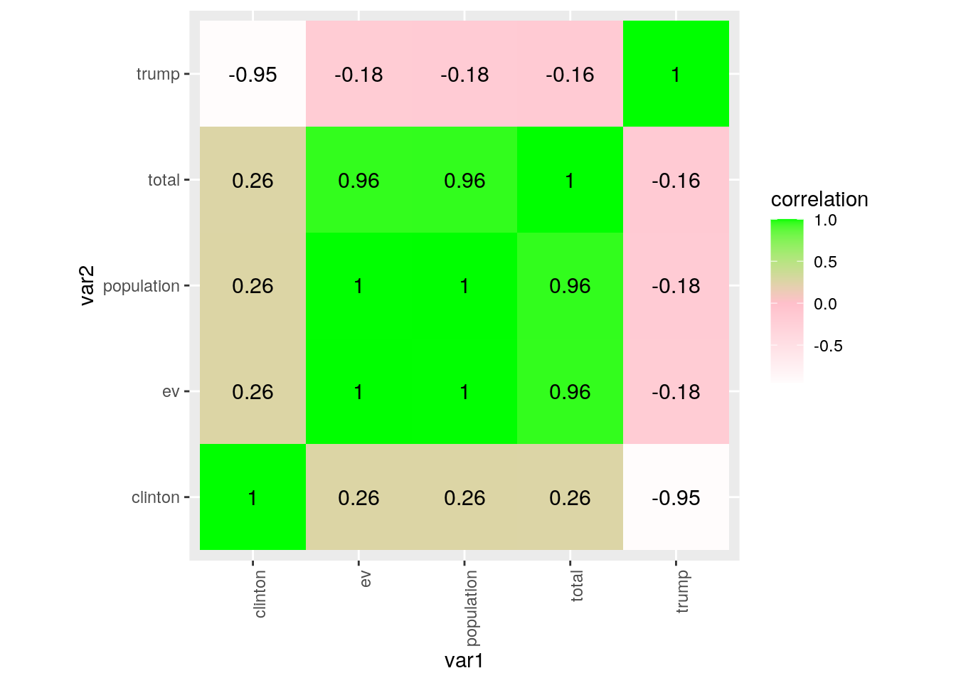
p <- project %>% ggplot(aes(population, total, label = abb, color = region)) +
    geom_label()
p + scale_x_log10() + scale_y_log10() + ggtitle("Gun murder data")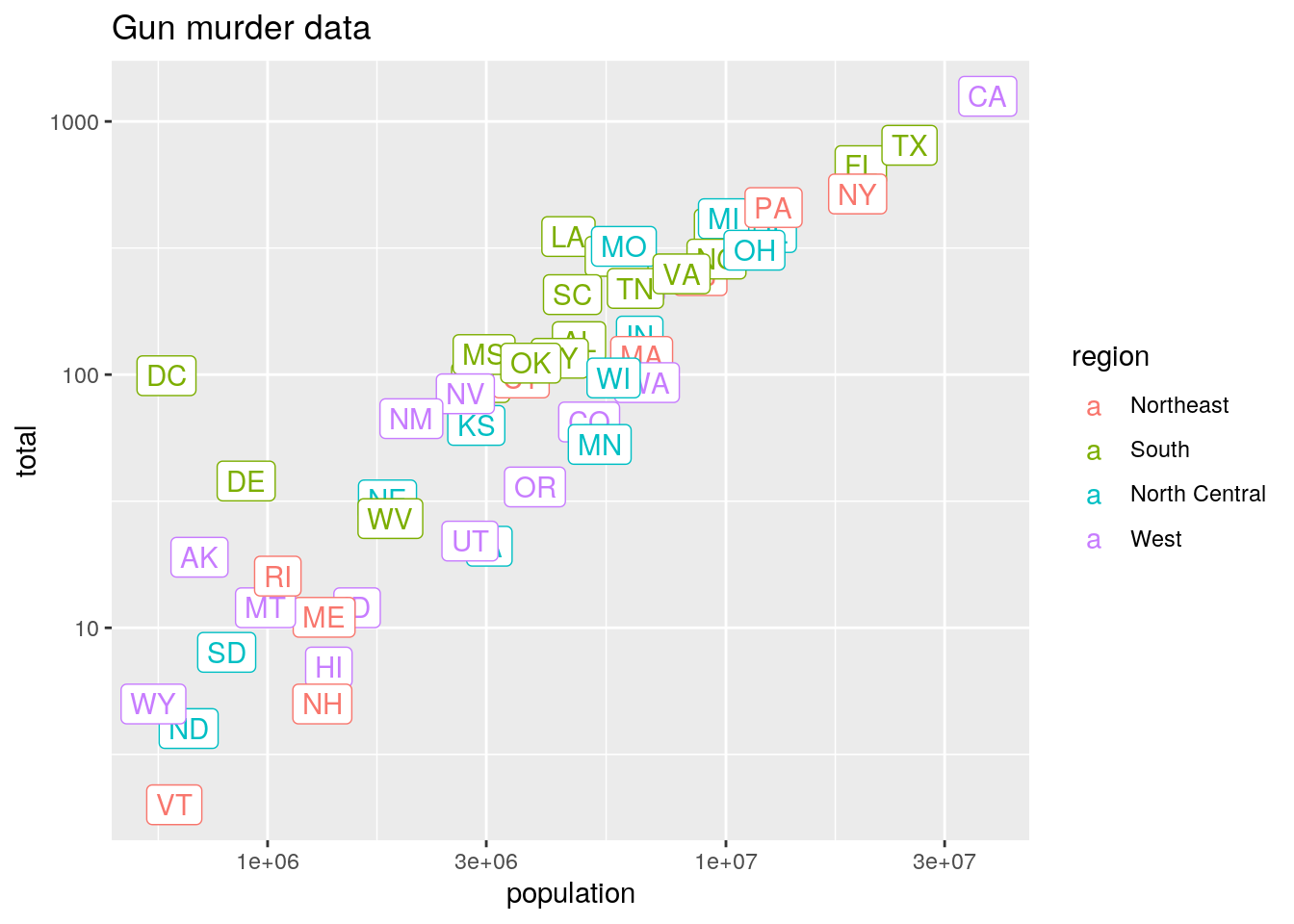
r <- murders %>% summarize(rate = sum(total)/sum(population) *
    10^6) %>% pull(rate)
project %>% ggplot(aes(population/10^6, total, label = abb)) +
    geom_abline(intercept = log10(r), lty = 2, color = "darkgrey") +
    geom_point(aes(col = region), size = 3) + scale_x_log10() +
    scale_y_log10() + xlab("Populations in millions (log scale)") +
    ylab("Total number of murders (log scale)") + ggtitle("US Gun Murders in 2010") +
    scale_color_discrete(name = "Region") + scale_x_continuous(breaks = round(seq(min(0),
    max(40), by = 5), 1)) + scale_y_continuous(breaks = round(seq(min(0),
    max(1100), by = 150), 1))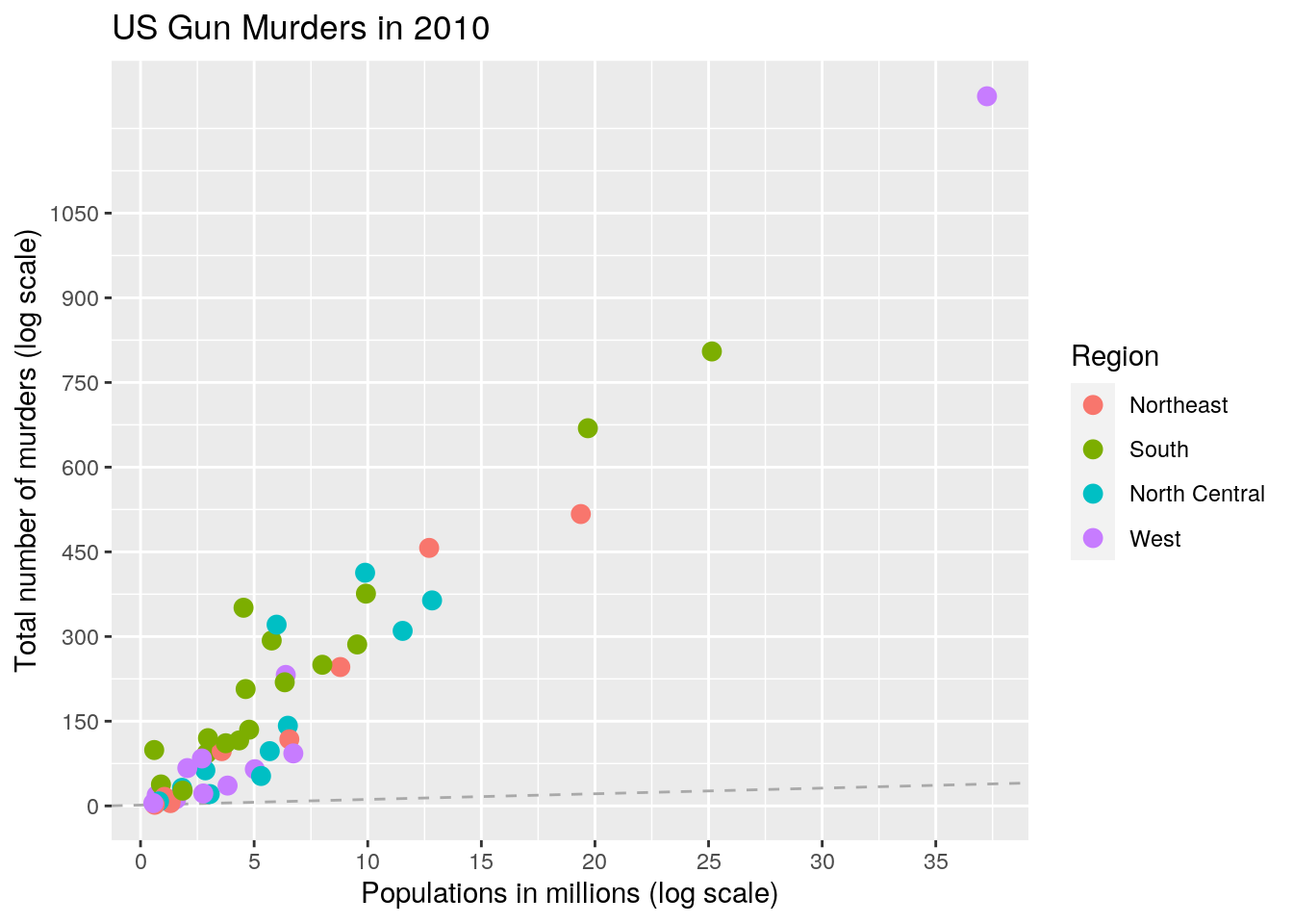
Clustering
library(tidyverse)
library(cluster)
# project
clust_dat <- project %>% select(population, trump, clinton)

set.seed(348)
kmeans1 <- clust_dat %>% kmeans(3)
kmeans1
## K-means clustering with 3 clusters of sizes 4, 16, 31
##
## Cluster means:
## population trump clinton
## 1 25366318 42.32500 52.92500
## 2 8321570 46.76875 48.04375
## 3 2427543 50.10968 42.05484
##
## Clustering vector:
## [1] 3 3 2 3 1 3 3 3 3 1 2 3 3 2 2 3 3 3 3 3 2 2 2 3 3 2 3 3 3 3 2 3 1 2 3 2 3 3
## [39] 2 3 3 3 2 1 3 3 2 2 3 2 3
##
## Within cluster sum of squares by cluster:
## [1] 2.094706e+14 9.222656e+13 6.994668e+13
## (between_SS / total_SS = 84.2 %)
##
## Available components:
##
## [1] "cluster" "centers" "totss" "withinss" "tot.withinss"
## [6] "betweenss" "size" "iter" "ifault"kmeansclust <- clust_dat %>% mutate(cluster = as.factor(kmeans1$cluster))
kmeansclust %>% ggplot(aes(trump, clinton, color = cluster)) +
geom_point()