Python/R Skills: Emma Uwakwe

January 1, 2022

Intro

In this individual project I chose to look at the efficiency of three different weight loss methods. There are binary values corresponding to either male or female, 0 and 1, respectively.

Significance Tests

library(readr)
diet <- read_csv("stcp-Rdataset-Diet.csv")

diet$weight.loss<-diet$pre.weight - diet$weight6weeks

man1<-manova(cbind(weight.loss,Age,pre.weight,Height)~Diet, data=diet)
summary(man1)

## Df Pillai approx F num Df den Df Pr(>F)
## Diet 1 0.11027 2.2618 4 73 0.07064 .
## Residuals 76
## ---
## Signif. codes: 0 '***' 0.001 '**' 0.01 '*' 0.05 '.' 0.1
' ' 1

summary.aov(man1)

## Response weight.loss :
## Df Sum Sq Mean Sq F value Pr(>F)
## Diet 1 45.78 45.781 7.6387 0.007164 **
## Residuals 76 455.49 5.993
## ---
## Signif. codes: 0 '***' 0.001 '**' 0.01 '*' 0.05 '.' 0.1
' ' 1
##
## Response Age :
## Df Sum Sq Mean Sq F value Pr(>F)
## Diet 1 121.0 120.984 1.26 0.2652
## Residuals 76 7297.2 96.015
##
## Response pre.weight :
## Df Sum Sq Mean Sq F value Pr(>F)
## Diet 1 9.0 9.019 0.1172 0.7331
## Residuals 76 5850.4 76.979
##
## Response Height :
## Df Sum Sq Mean Sq F value Pr(>F)
## Diet 1 136.9 136.90 1.0776 0.3025
## Residuals 76 9654.6 127.03

diet%>%group_by(Diet)%>%summarize(mean(weight.loss))

## # A tibble: 3 x 2
##    Diet `mean(weight.loss)`
##   <dbl>               <dbl>
## 1     1                3.3 
## 2     2                3.03
## 3     3                5.15

pairwise.t.test(diet$weight.loss,diet$Diet, p.adj="none")

## 
##  Pairwise comparisons using t tests with pooled SD 
## 
## data:  diet$weight.loss and diet$Diet 
## 
##   1      2     
## 2 0.6845 -     
## 3 0.0075 0.0017
## 
## P value adjustment method: none

I performed 8 tests, one multivariate MANOVA, 4 ANOVA, and 3 post hoc T-tests, with an alpha of .0063. My F statistic was not significant. I proceeded to do a follow-up univariate ANOVA, which showed that the relationship between diet and weight loss was significant, with a statistic of .006. I then performed Post hoc analysis by conducting pairwise comparisons to determine which diets differed in weight loss.

Randomization Test

diet%>%group_by(Diet)%>%summarize(mean=mean(weight.loss))

## # A tibble: 3 x 2
##    Diet  mean
##   <dbl> <dbl>
## 1     1  3.3 
## 2     2  3.03
## 3     3  5.15

diet%>%group_by(Diet)%>%summarize(s=sd(weight.loss))

## # A tibble: 3 x 2
##    Diet     s
##   <dbl> <dbl>
## 1     1  2.24
## 2     2  2.52
## 3     3  2.40

diet%>%group_by(Diet)%>%summarize(n())

## # A tibble: 3 x 2
##    Diet `n()`
##   <dbl> <int>
## 1     1    24
## 2     2    27
## 3     3    27

df_two <- data.frame(loss = rnorm(25, mean=3.268000 , sd=2.464535),Diet = "2")
df_three <- data.frame(loss = rnorm(27, mean=5.148148, sd=2.395568  ),Diet="3")

df_weight_loss <- rbind(df_two, df_three)

ggplot(df_weight_loss, aes(x = loss, fill = Diet)) + ylab("Count") + xlab("Weight Loss") + geom_histogram(bins = 30, colour = "black") + 
  geom_vline(data = filter(df_weight_loss, Diet == "2"), aes(xintercept = mean(loss)),size = 1, linetype = "dashed", colour = "green") + geom_vline(data = filter(df_weight_loss, Diet == "3"), aes(xintercept = mean(loss)),size = 1, linetype = "dashed", colour = "blue")+theme_classic()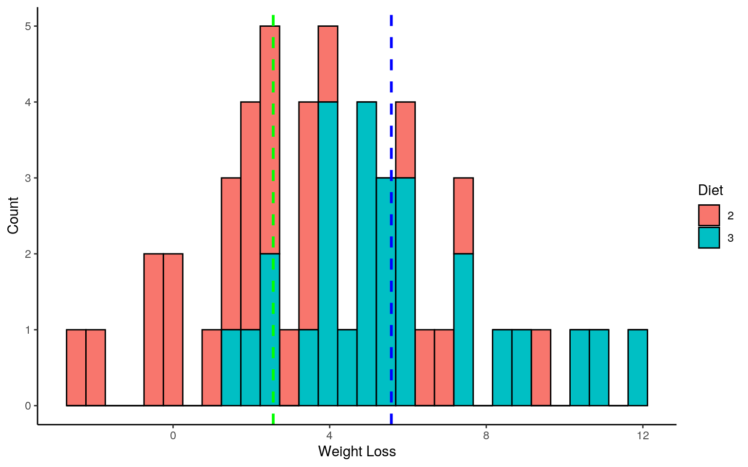

mean_two <- mean(df_two$loss)
mean_three <- mean(df_three$loss)
diff_means_obs <- mean_three - mean_two

t.test(loss ~ Diet, data = df_weight_loss, alternative = "two.sided")

##
## Welch Two Sample t-test
##
## data: loss by Diet
## t = -3.8982, df = 48.558, p-value = 0.000297
## alternative hypothesis: true difference in means is not
equal to 0
## 95 percent confidence interval:
## -4.573266 -1.461555
## sample estimates:
## mean in group 2 mean in group 3
## 2.557799 5.575210

set.seed(49)
simulated_means <- list()
nreps = 5000
for(i in 1:nreps){
        reshuffled <- df_weight_loss
reshuffled$loss <- sample(reshuffled$loss, 
                           size = nrow(reshuffled), replace = FALSE)
mean_diet_2_sim<- mean(reshuffled %>% filter(Diet == "2") %>% pull(loss))
mean_diet_3_sim<- mean(reshuffled %>% filter(Diet == "3") %>% pull(loss))

mean_diff_sim <- mean_diet_3_sim - mean_diet_2_sim
    
simulated_means[i] <- mean_diff_sim
}    
simulated_means <- unlist(simulated_means)

simulated_means[1:10]

## [1] 0.95573647 -0.49833031 0.07062388 0.27616359
-0.90648121 0.25392773 -0.52665208 -0.51084717
## [9] -1.38985738 -0.81178937

ggplot() + ylab("Count") + xlab("Simulated mean weight loss difference") +
    geom_histogram(aes(x = simulated_means), bins = 30, 
                   fill = "grey", alpha = 0.4, colour = "black") +
    geom_vline(xintercept = diff_means_obs, size = 1, 
               linetype = "dashed", colour = "black") + 
    theme_classic()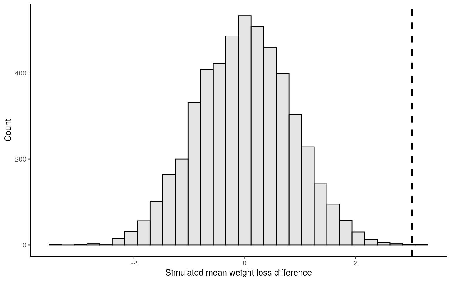

abs_simulated_means <- abs(simulated_means)
abs_diff_means_obs <- abs(diff_means_obs)
exceed_count <- length(abs_simulated_means[abs_simulated_means >= 
                                               abs_diff_means_obs])
p_val <- exceed_count / nreps
view(p_val)

Linear Regression

center_scale <- function(x) {scale(x, scale = FALSE)}
diet$age_scaled<-center_scale(diet$Age)
diet$weightloss_scaled<-center_scale(diet$weight.loss)
diet$height_scaled<-center_scale(diet$Height)

fit<-lm(weightloss_scaled ~ age_scaled * height_scaled, data=diet)
summary(fit)

##
## Call:
## lm(formula = weightloss_scaled ~ age_scaled *
height_scaled,
## data = diet)
##
## Residuals:
## Min 1Q Median 3Q Max
## -5.783 -1.701 -0.085 1.582 5.286
##
## Coefficients:
## Estimate Std. Error t value Pr(>|t|)
## (Intercept) 0.031269 0.290551 0.108 0.915
## age_scaled -0.020978 0.030521 -0.687 0.494
## height_scaled -0.011604 0.028219 -0.411 0.682
## age_scaled:height_scaled -0.003560 0.002902 -1.227 0.224
##
## Residual standard error: 2.556 on 74 degrees of freedom
## Multiple R-squared: 0.03541, Adjusted R-squared:
-0.003693
## F-statistic: 0.9056 on 3 and 74 DF, p-value: 0.4426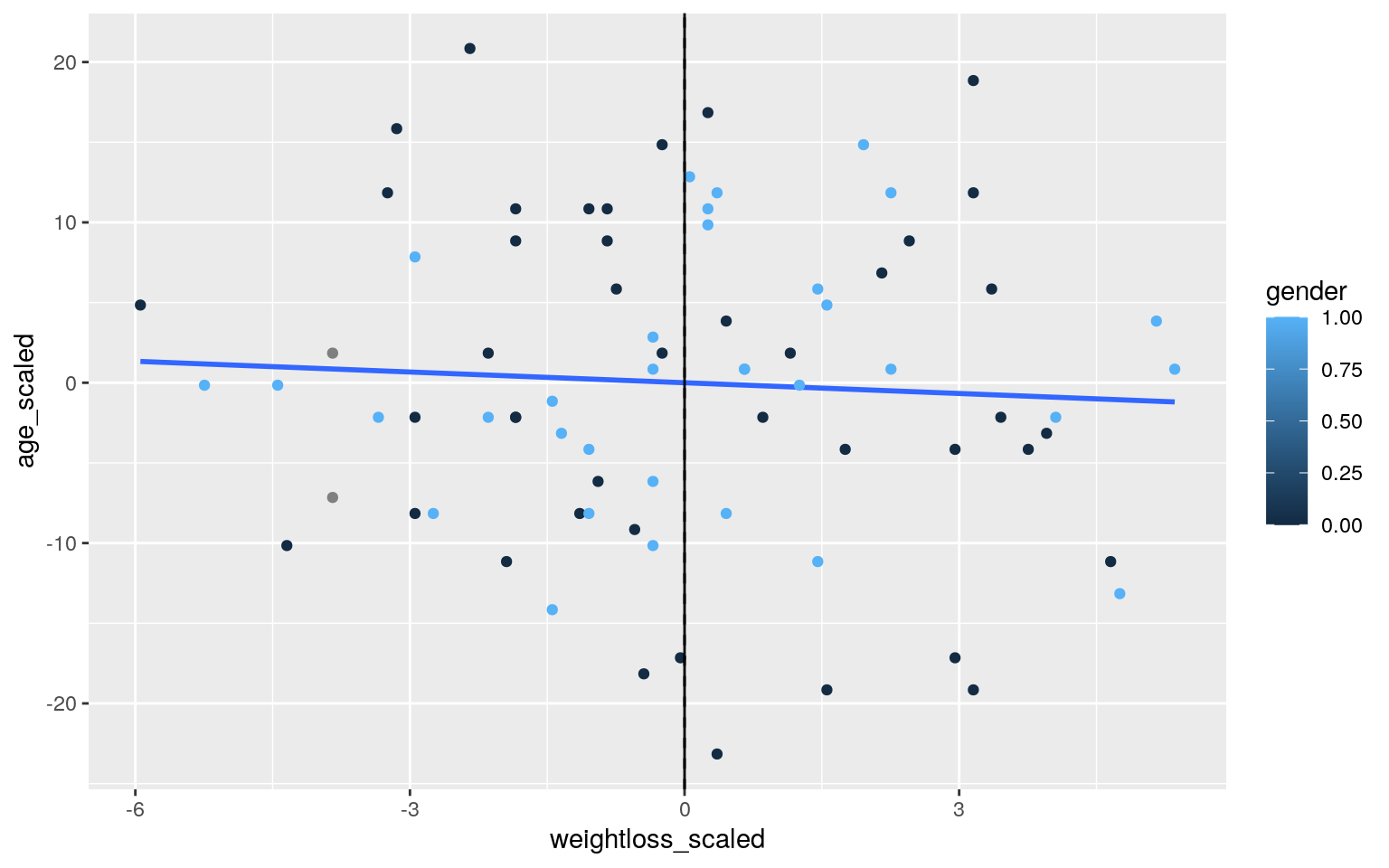

library(interactions) #interact_plot(fit,weightloss_scaled,height_scaled) ggplot(diet, aes(weightloss_scaled,age_scaled, color = gender)) +geom_smooth(method = "lm", se = F, fullrange = T)+ geom_point()+geom_vline(xintercept=0,lty=2)+geom_vline(xintercept=mean(diet$weightloss_scaled))

plot(fit,1)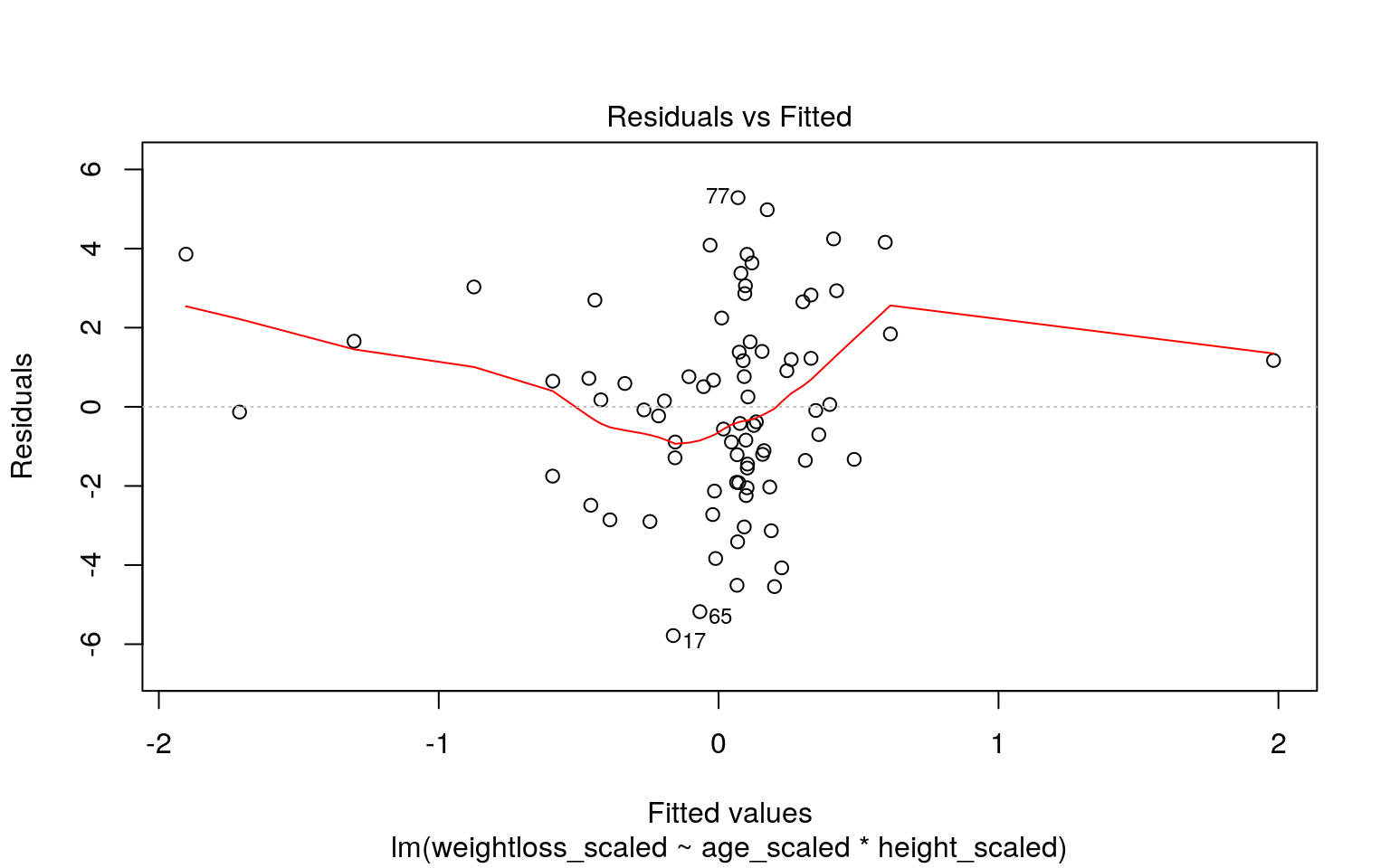

plot(fit, 3)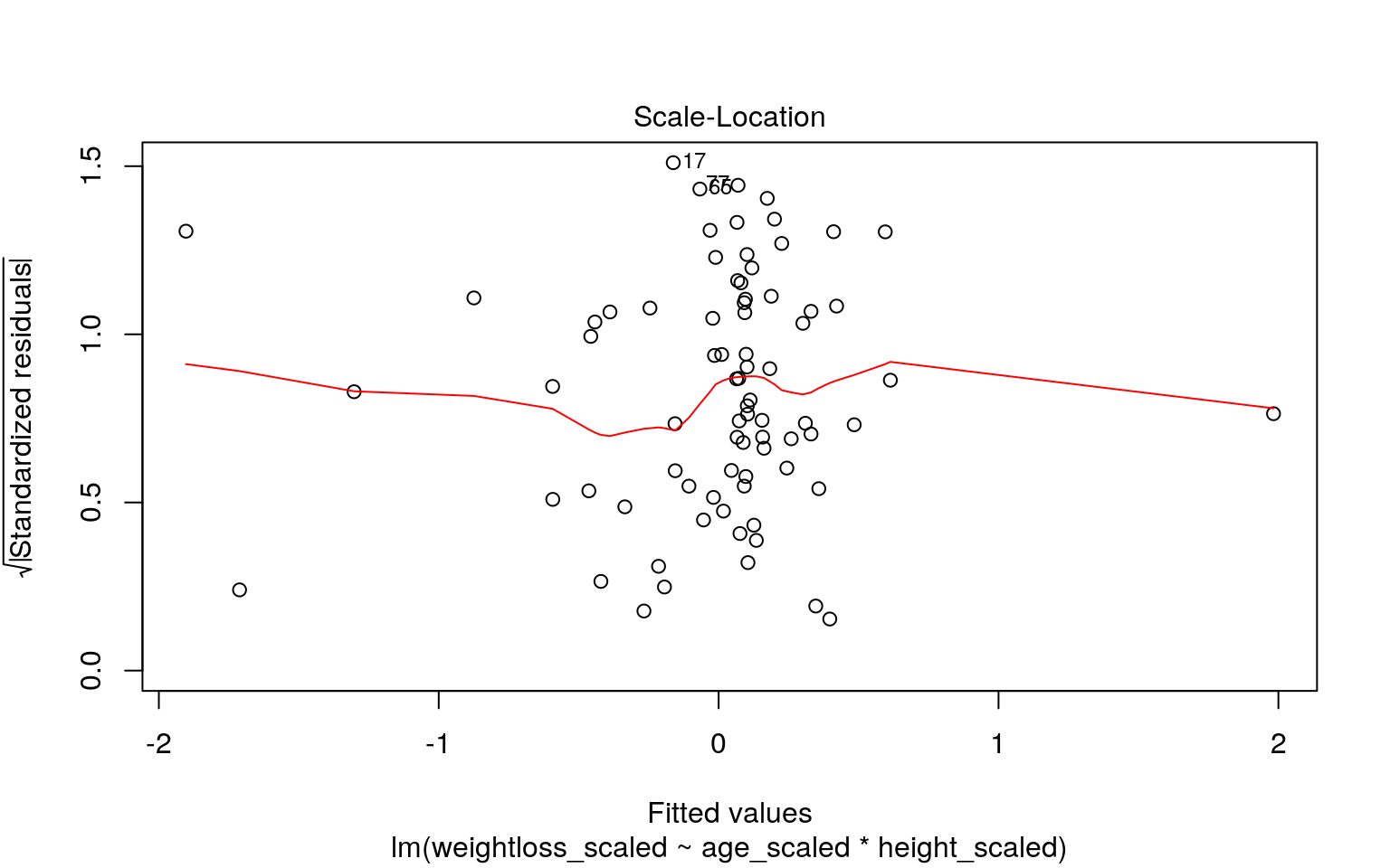

plot(fit, 2)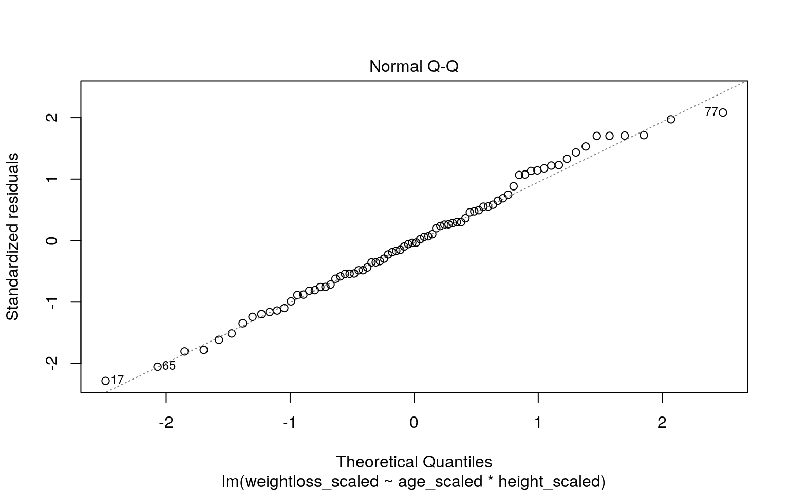

library(lmtest)
library(car)
library(sandwich)
coeftest(fit, vcov = vcovHC(fit))[,1:2]

##                             Estimate  Std. Error
## (Intercept)               0.03126928 0.298750582
## age_scaled               -0.02097818 0.029870458
## height_scaled            -0.01160375 0.028090352
## age_scaled:height_scaled -0.00355979 0.003000632

Bootstrapping

fit<-lm(weightloss_scaled ~ age_scaled*height_scaled, data=diet)
resids<-fit$residuals
fitted<-fit$fitted.values

resid_resamp<-replicate(5000,{
new_resids<-sample(resids,replace=TRUE) 
diet$new_y<-fitted+new_resids 
fit<-lm(new_y~age_scaled *height_scaled,data=diet) 
coef(fit) 
})

resid_resamp%>%t%>%as.data.frame%>%summarize_all(sd)

## (Intercept) age_scaled height_scaled
age_scaled:height_scaled
## 1 0.2836641 0.02969396 0.02787081 0.002804571

Logistic Modeling

library(tidyverse)
library(lmtest)
fit3<-glm(gender~Height + pre.weight,data=diet,family=binomial)
summary(fit3)

##
## Call:
## glm(formula = gender ~ Height + pre.weight, family =
binomial,
## data = diet)
##
## Deviance Residuals:
## Min 1Q Median 3Q Max
## -2.51852 -0.31321 -0.07863 0.34234 2.25270
##
## Coefficients:
## Estimate Std. Error z value Pr(>|z|)
## (Intercept) -44.69997 10.78914 -4.143 3.43e-05 ***
## Height 0.08002 0.03660 2.187 0.0288 *
## pre.weight 0.42030 0.09960 4.220 2.44e-05 ***
## ---
## Signif. codes: 0 '***' 0.001 '**' 0.01 '*' 0.05 '.' 0.1
' ' 1
##
## (Dispersion parameter for binomial family taken to be 1)
##
## Null deviance: 104.039 on 75 degrees of freedom
## Residual deviance: 40.182 on 73 degrees of freedom
## (2 observations deleted due to missingness)
## AIC: 46.182
##
## Number of Fisher Scoring iterations: 6

exp(coef(fit3))

##  (Intercept)       Height   pre.weight 
## 3.864094e-20 1.083314e+00 1.522415e+00

class_diag<-function(probs,truth){ if(is.numeric(truth)==FALSE & is.logical(truth)==FALSE) truth<-as.numeric(truth)-1 prediction<-ifelse(probs>.5,1,0) acc=mean(truth==prediction) sens=mean(prediction[truth==1]==1) spec=mean(prediction[truth==0]==0) ppv=mean(truth[prediction==1]==1) f1=2*(sens*ppv)/(sens+ppv) #CALCULATE EXACT AUC ord<-order(probs, decreasing=TRUE) probs <- probs[ord]; truth <- truth[ord] TPR=cumsum(truth)/max(1,sum(truth)) FPR=cumsum(!truth)/max(1,sum(!truth)) dup<-c(probs[-1]>=probs[-length(probs)], FALSE) TPR<-c(0,TPR[!dup],1); FPR<-c(0,FPR[!dup],1) n <- length(TPR) auc<- sum( ((TPR[-1]+TPR[-n])/2) * (FPR[-1]-FPR[-n]) ) data.frame(acc,sens,spec,ppv,auc) } gen<-as.numeric(fit3$y)%>%na.omit() PROBS<-predict(fit3,type = "response")%>%na.omit table(predict=as.numeric(PROBS>.5),truth=gen)%>%addmargins

##        truth
## predict  0  1 Sum
##     0   40  3  43
##     1    3 30  33
##     Sum 43 33  76

#Accuracy: (40+30)/76 = .921,  92.1% of cases are classified correctly 
#Sensitivity: 30/33 = .090, 9% of men are correctly classified
#Specificity: 40/43 = .930, 93% of women are correctly classified
#Precsion: 40/43 = .930, woman who are classified as woman who actually are
#AUC : 0.9556025, easy to predict gender from height and pre weight 

library(plotROC)
ROCplot<-ggplot(fit3)+geom_roc(aes(d=fit3$y,m=PROBS), n.cuts=0)
ROCplot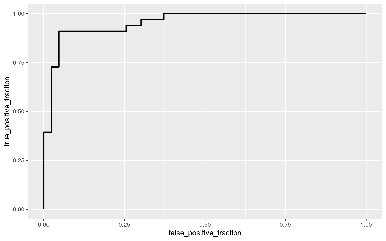

calc_auc(ROCplot)

##   PANEL group       AUC
## 1     1    -1 0.9556025

#diet%>%ggplot(aes(diet$logit,color=gender,fill=gender))+geom_density(alpha=.4)+theme(legend.position=c(.85,.85))+geom_vline(xintercept=0)+xlab("predictor (logit)")

Logistical Modeling Part 2

fit4<-glm(gender ~., data = diet, family = "binomial")
summary(fit4)

##
## Call:
## glm(formula = gender ~ ., family = "binomial", data =
diet)
##
## Deviance Residuals:
## Min 1Q Median 3Q Max
## -3.514e-05 -2.100e-08 -2.100e-08 2.100e-08 2.882e-05
##
## Coefficients: (4 not defined because of singularities)
## Estimate Std. Error z value Pr(>|z|)
## (Intercept) 4.913e+02 6.121e+05 0.001 0.999
## Person 1.641e+01 1.157e+04 0.001 0.999
## Age 6.888e-01 5.998e+03 0.000 1.000
## Height 1.562e-01 1.388e+03 0.000 1.000
## pre.weight -7.623e+00 1.304e+04 -0.001 1.000
## Diet -4.220e+02 3.011e+05 -0.001 0.999
## weight6weeks 2.762e+00 1.093e+04 0.000 1.000
## weight.loss NA NA NA NA
## age_scaled NA NA NA NA
## weightloss_scaled NA NA NA NA
## height_scaled NA NA NA NA
##
## (Dispersion parameter for binomial family taken to be 1)
##
## Null deviance: 1.0404e+02 on 75 degrees of freedom
## Residual deviance: 3.7770e-09 on 69 degrees of freedom
## (2 observations deleted due to missingness)
## AIC: 14
##
## Number of Fisher Scoring iterations: 25

exp(coef(fit4))

## (Intercept) Person Age Height pre.weight
## 2.231405e+213 1.340347e+07 1.991313e+00 1.169093e+00
4.889389e-04
## Diet weight6weeks weight.loss age_scaled
weightloss_scaled
## 5.137349e-184 1.582470e+01 NA NA NA
## height_scaled
## NA

gen2<-as.numeric(fit4$y)%>%na.omit()
PROBS2<-predict(fit4,type = "response")%>%na.omit
class_diag(PROBS2,gen2)

##   acc sens spec ppv auc
## 1   1    1    1   1   1

library(glmnet)
library(dplyr)
diet2<-diet

#folding part 1
set.seed(1234)
k=10
data <- diet2 %>% sample_frac #put rows of dataset in random order
folds <- ntile(1:nrow(data),n=10) #create fold labels
diags<-NULL
for(i in 1:k){
train <- data[folds!=i,] #create training set (all but fold i)
test <- data[folds==i,] #create test set (just fold i)
truth <- diet2$gender #save truth labels from fold i
fit5 <- glm(gender~(.)^2, data=train, family="binomial")
probs <- predict(fit5, newdata=test, type="response")
diags<-rbind(diags,class_diag(probs,truth))
}
class_diag(probs,truth)

##   acc sens spec ppv auc
## 1  NA   NA   NA  NA  NA

#lasso
diet2<-diet
gen3<-as.numeric(fit4$y)%>%na.omit()
yes <- as.matrix(gen3) 
xes<-model.matrix(gender~. ,data=diet2)[,-1]
xes<-scale(xes)
cv <- cv.glmnet(xes, yes, family = "binomial") 
lasso <- glmnet(xes, yes, family = "binomial", lambda = cv$lamda.1se)
#coef(lasso) #Values that show up are the most predictive variables

#Folding part 2
fit6<-glm(gender ~ Height + pre.weight, data = diet2, family = "binomial")
set.seed(1234)
k=10
data <- diet2 %>% sample_frac #put rows of dataset in random order
folds <- ntile(1:nrow(data),n=10) #create fold labels
diags<-NULL
for(i in 1:k){
train2 <- data[folds!=i,] #create training set (all but fold i)
test2 <- data[folds==i,] #create test set (just fold i)
truth2 <- diet2$gender #save truth labels from fold i
fit7 <- glm(gender~Height + pre.weight, data=train, family="binomial")
probs2 <- predict(fit7, newdata=test2, type="response")
diags2<-rbind(diags,class_diag(probs2,truth2))
}
class_diag(probs2,truth2)

##   acc sens spec ppv auc
## 1  NA   NA   NA  NA  NA